I’m trying to understand nonparametric statistics a little more formally. This post may not be that intelligible because I’m still pretty confused about nonparametric statistics, there is a lot of math, and I make no attempt to explain any of the math notation. I’m working towards being able to explain this stuff in a much more accessible way but first I would like to understand some of the math!

There’s some MathJax in this post so the math may or may not render in an RSS reader.

Some questions I’m interested in:

• what is nonparametric statistics exactly?
• what guarantees can we make? are there formulas we can use?
• why do methods like the bootstrap method work?

since these notes are from reading a math book and math books are extremely dense this is basically going to be “I read 7 pages of this math book and here are some points I’m confused about”

what’s nonparametric statistics?

Today I’m looking at “all of nonparametric statistics” by Larry Wasserman. He defines nonparametric inference as:

a set of modern statistical methods that aim to keep the number of underlying assumptions as weak as possible

Basically my interpretation of this is that – instead of assuming that your data comes from a specific family of distributions (like the normal distribution) and then trying to estimate the parameters of that distribution, you don’t make many assumptions about the distribution (“this is just some data!!”). Not having to make assumptions is nice!

There aren’t no assumptions though – he says

we assume that the distribution $F$ lies in some set $\mathfrak{F}$ called a statistical model. For example, when estimating a density $f$, we might assume that $$ f \in \mathfrak{F} = \left\{ g : \int(g^{\prime\prime}(x))^2dx \leq c^2 \right\}$$ which is the set of densities that are not “too wiggly”.

I have not too much intuition for the condition $\int(g^{\prime\prime}(x))^2dx \leq c^2$. I calculated that integral for the normal distribution on wolfram alpha and got 4, which is a good start. (4 is not infinity!)

some questions I still have about this definition:

• what’s an example of a probability density function that doesn’t satisfy that $\int(g^{\prime\prime}(x))^2dx \leq c^2$ condition? (probably something with an infinite number of tiny wiggles, and I don’t think any distribution i’m interested in in practice would have an infinite number of tiny wiggles?)
• why does the density function being “too wiggly” cause problems for nonparametric inference? very unclear as yet.

we still have to assume independence

One assumption we won’t get away from is that the samples in the data we’re dealing with are independent. Often data in the real world actually isn’t really independent, but I think the what people do a lot of the time is to make a good effort at something approaching independence and then close your eyes and pretend it is?

estimating the density function

Okay! Here’s a useful section! Let’s say that I have 100,000 data points from a distribution. I can draw a histogram like this of those data points:

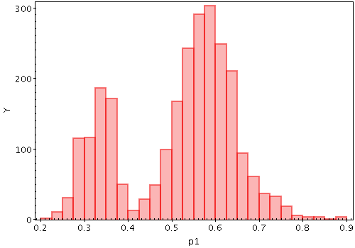
If I have 100,000 data points, it’s pretty likely that that histogram is pretty close to the actual distribution. But this is math, so we should be able to make that statement precise, right?

For example suppose that 5% of the points in my sample are more than 100. Is the probability that a point is greater than 100 actually 0.05? The book gives a nice formula for this:

$$ \mathbb{P}(|\widehat{P}_n(A) - P(A)| > \epsilon ) \leq 2e^{-2n\epsilon^2} $$

(by “Hoeffding’s inequality” which I’ve never heard of before). Fun aside about that inequality: here’s a nice jupyter notebook by henry wallace using it to identify the most common Boggle words.

here, in our example:

• n is 1000 (the number of data points we have)
• $A$ is the set of points more than 100
• $\widehat{P}_n(A)$ is the empirical probability that a point is more than 100 (0.05)
• $P(A)$ is the actual probability
• $\epsilon$ is how certain we want to be that we’re right

So, what’s the probability that the real probability is between 0.04 and 0.06? $\epsilon = 0.01$, so it’s $2e^{-2 \times 100,000 \times (0.01)^2} = 4e^{-9} $ ish (according to wolfram alpha)

here is a table of how sure we can be:

• 100,000 data points: 4e-9 (TOTALLY CERTAIN that 4% - 6% of points are more than 100)
• 10,000 data points: 0.27 (27% probability that we’re wrong! that’s… not bad?)
• 1,000 data points: 1.6 (we know the probability we’re wrong is less than.. 160%? that’s not good!)
• 100 data points: lol

so basically, in this case, using this formula: 100,000 data points is AMAZING, 10,000 data points is pretty good, and 1,000 is much less useful. If we have 1000 data points and we see that 5% of them are more than 100, we DEFINITELY CANNOT CONCLUDE that 4% to 6% of points are more than 100. But (using the same formula) we can use $\epsilon = 0.04$ and conclude that with 92% probability 1% to 9% of points are more than 100. So we can still learn some stuff from 1000 data points!

This intuitively feels pretty reasonable to me – like it makes sense to me that if you have NO IDEA what your distribution that with 100,000 points you’d be able to make quite strong inferences, and that with 1000 you can do a lot less!

more data points are exponentially better?

One thing that I think is really cool about this estimating the density function formula is that how sure you can be of your inferences scales exponentially with the size of your dataset (this is the $e^{-n\epsilon^2}$). And also exponentially with the square of how sure you want to be (so wanting to be sure within 0.01 is VERY DIFFERENT than within 0.04). So 100,000 data points isn’t 10x better than 10,000 data points, it’s actually like 10000000000000x better.

Is that true in other places? If so that seems like a super useful intuition! I still feel pretty uncertain about this, but having some basic intuition about “how much more useful is 10,000 data points than 1,000 data points?”) feels like a really good thing.

some math about the bootstrap

The next chapter is about the bootstrap! Basically the way the bootstrap works is:

1. you want to estimate some statistic (like the median) of your distribution
2. the bootstrap lets you get an estimate and also the variance of that estimate
3. you do this by repeatedly sampling with replacement from your data and then calculating the statistic you want (like the median) on your samples

I’m not going to go too much into how to implement the bootstrap method because it’s explained in a lot of place on the internet. Let’s talk about the math!

I think in order to say anything meaningful about bootstrap estimates I need to learn a new term: a consistent estimator.

What’s a consistent estimator?

Wikipedia says:

In statistics, a consistent estimator or asymptotically consistent estimator is an estimator — a rule for computing estimates of a parameter $\theta_0$ — having the property that as the number of data points used increases indefinitely, the resulting sequence of estimates converges in probability to $\theta_0$.

This includes some terms where I forget what they mean (what’s “converges in probability” again?). But this seems like a very good thing! If I’m estimating some parameter (like the median), I would DEFINITELY LIKE IT TO BE TRUE that if I do it with an infinite amount of data then my estimate works. An estimator that is not consistent does not sound very useful!

why/when are bootstrap estimators consistent?

spoiler: I have no idea. The book says the following:

Consistency of the boostrap can now be expressed as follows.

3.19 Theorem. Suppose that $\mathbb{E}(X_1^2) < \infty$. Let $T_n = g(\overline{X}_n)$ where $g$ is continuously differentiable at $\mu = \mathbb{E}(X_1)$ and that $g\prime(\mu) \neq 0$. Then,

$$ \sup_u | \mathbb{P}_{\widehat{F}_n} \left( \sqrt{n} (T( \widehat{F}_n*) - T( \widehat{F}_n) \leq u \right) - \mathbb{P}_{\widehat{F}} \left( \sqrt{n} (T( \widehat{F}_n) - T( \widehat{F}) \leq u \right) | \rightarrow^\text{a.s.} 0 $$

3.21 Theorem. Suppose that $T(F)$ is Hadamard differentiable with respect to $d(F,G)= sup_x|F(x)-G(x)|$ and that $0 < \int L^2_F(x) dF(x) < \infty$. Then,

$$ \sup_u | \mathbb{P}_{\widehat{F}_n} \left( \sqrt{n} (T( \widehat{F}_n*) - T( \widehat{F}_n) \leq u \right) - \mathbb{P}_{\widehat{F}} \left( \sqrt{n} (T( \widehat{F}_n) - T( \widehat{F}) \leq u \right) | \rightarrow^\text{P} 0 $$

things I understand about these theorems:

• the two formulas they’re concluding are the same, except I think one is about convergence “almost surely” and one about “convergence in probability”. I don’t remember what either of those mean.
• I think for our purposes of doing Regular Boring Things we can replace “Hadamard differentiable” with “differentiable”
• I think they don’t actually show the consistency of the bootstrap, they’re actually about consistency of the bootstrap confidence interval estimate (which is a different thing)

I don’t really understand how they’re related to consistency, and in particular the $\sup_u$ thing is weird, like if you’re looking at $\mathbb{P}(something < u)$, wouldn’t you want to minimize $u$ and not maximize it? Maybe it’s a typo and it should be $\inf_u$?

it concludes:

there is a tendency to treat the bootstrap as a panacea for all problems. But the bootstrap requires regularity conditions to yield valid answers. It should not be applied blindly.

this book does not seem to explain why the bootstrap is consistent

In the appendix (3.7) it gives a sketch of a proof for showing that estimating the median using the bootstrap is consistent. I don’t think this book actually gives a proof anywhere that bootstrap estimates in general are consistent, which was pretty surprising to me. It gives a bunch of references to papers. Though I guess bootstrap confidence intervals are the most important thing?

that’s all for now

This is all extremely stream of consciousness and I only spent 2 hours trying to work through this, but some things I think I learned in the last couple hours are:

1. maybe having more data is exponentially better? (is this true??)
2. “consistency” of an estimator is a thing, not all estimators are consistent
3. understanding when/why nonparametric bootstrap estimators are consistent in general might be very hard (the proof that the bootstrap median estimator is consistent already seems very complicated!)
4. boostrap confidence intervals are not the same thing as bootstrap estimators. Maybe I’ll learn the difference next!